2.2 Data Types
As a practitioner of data or someone who works with data, it is important to understand the different types of data. Intuitively, this makes sense: we understand that someone’s height is fundamentally different information from their blood pressure, favourite vegetable, or their name. We also understand that these different kinds of data cannot be directly compared.
As an example, consider two friends, Shamila and Kagiso. Shamila is 160cm tall, has a systolic blood pressure of 110, and likes broccoli. Kagiso is 180cm tall, has a systolic blood pressure of 119, and likes carrots. We can say that Kagiso is taller than Shamila, but we cannot say that Kagiso is taller than his blood pressure. We can say that Kagiso’s blood pressure is higher than Shamila’s, but we cannot say that Kagiso’s blood pressure is higher than broccoli (what would that even mean?). These differences may seem obvious in this example, but keep them in mind as we explore the different data types and scales of measurement.
2.2.1 Scales of Measurement
Scales of measurement refers to the categories in which we divide data according to their properties, and which inform the appropriate kinds of analyses we can perform on the data. There are four scales of measurement, namely nominal, ordinal, interval and ratio.
Consider the following dataset which is an extension of the dataset in Table 1 introduced in Section 1.2:
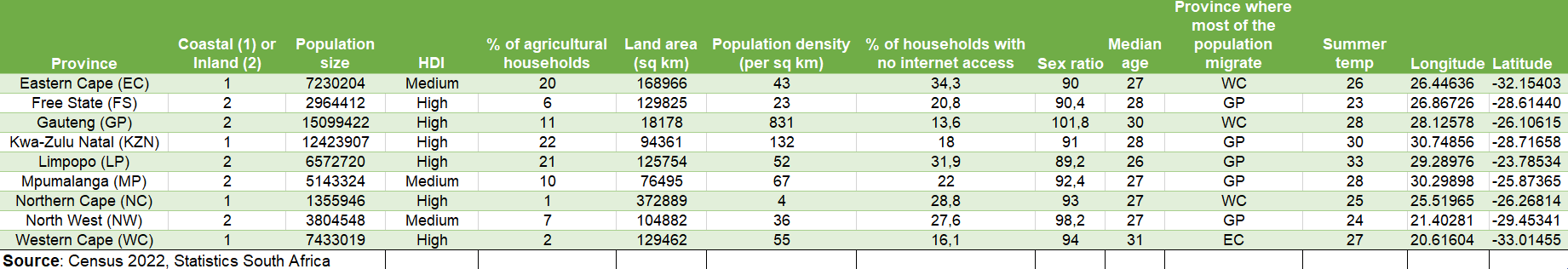
Figure 2.1: Provinces dataset
2.2.1.1 Nominal
Nominal data refers to data to which there is no order or ranking. In the Provinces dataset, there are three nominal variables. Province is a nominal variable, since there is no specific order to the provinces. Province where most of the population migrate is similarly a nominal variable.
Q: What is the third nominal variable in the Provinces dataset?
Nominal data is best represented by bar charts and pie charts.
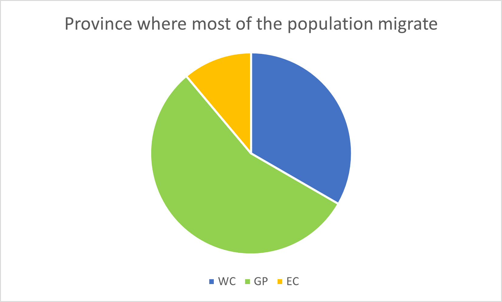
Figure 2.2: Pie chart of the ‘Province where most of the population migrate’ nominal variable.
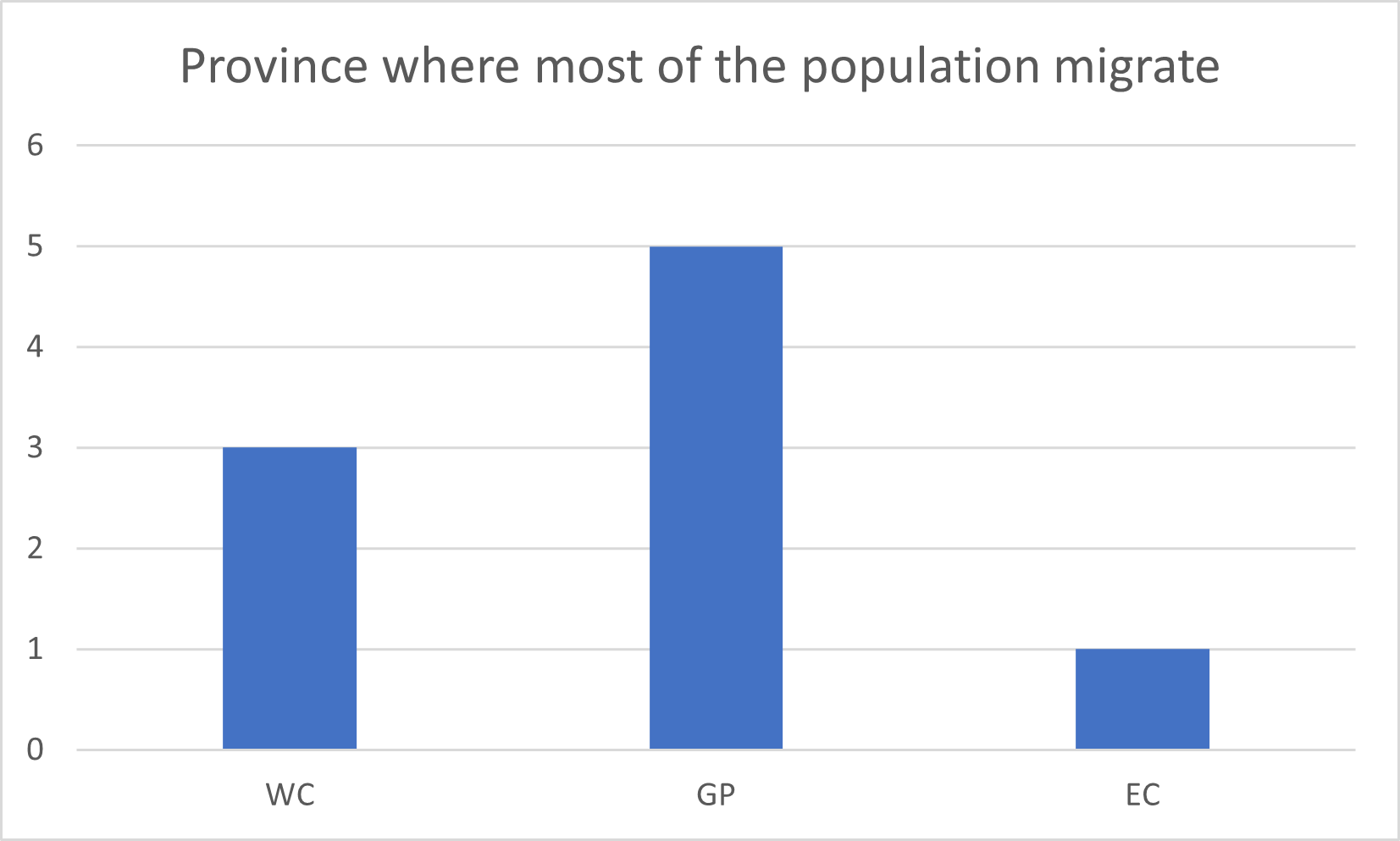
Figure 2.3: Bar chart of the ‘Province where most of the population migrate’ nominal variable.
Q: Would it be useful to make a pie chart or a bar chart of the Province variable? Why or why not?
2.2.1.2 Ordinal
Ordinal data refers to data that has an order, but where the difference in order cannot be measured. In the Provinces dataset, HDI (Human Development Index) is an ordinal variable. There is a clear order to the values of HDI, namely Medium or High. However, the difference in order cannot be measured quantitatively. We cannot, for instance, say that the Free State’s HDI is “twice as medium” as that of the Eastern Cape, or that North West’s HDI is “a third as high” as that of Western Cape.
Q: Can you think of other examples of ordinal variables?
Ordinal data is best represented by bar charts.
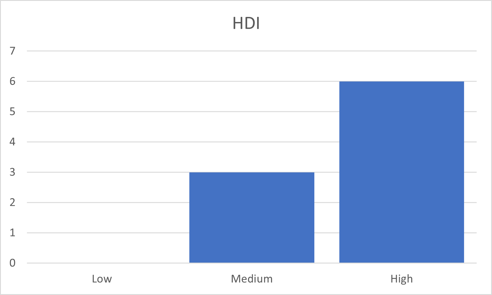
Figure 2.4: Bar chart of the ‘HDI’ ordinal variable.
2.2.1.3 Interval
Interval data refers to data that has an order, and where the difference in order can be measured, i.e. it can be quantified by a numerical value. However, the ratio between interval data values does not have a meaning, and there is no true zero. In the Provinces dataset, Summer temp is an interval-valued variable. This is because temperature does not have a true zero value. A temperature of 0 degrees Celsius is cold; it does not mean that there is no temperature.
Interval data can be represented by, among other things, bar charts, histograms, and box plots.
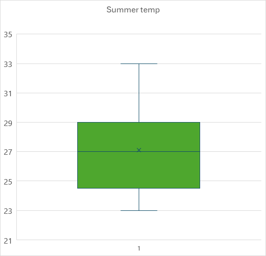
Figure 2.5: Box plot of the ‘Summer temp’ interval variable.
Q: Can you think of other examples of interval variables?
2.2.1.4 Ratio
Ratio data refers to data that has an order, where the difference in order can be measured quantitatively, and where the ratio between values has a meaning. The data also has a true zero. In the Provinces dataset, Land area, Population density, and % of agricultural households are examples of ratio variables.
Like interval data, ratio data can be represented by, among other things, bar charts, histograms, and box plots.
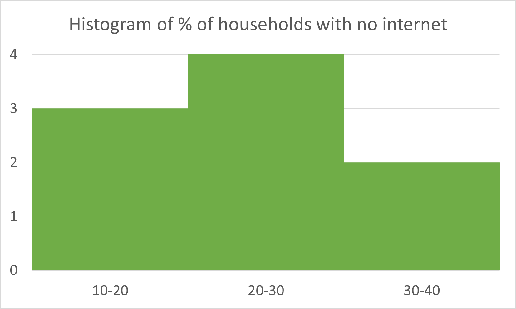
Figure 2.6: Histogram of the ‘% of households with no internet’ ratio variable.
Q: Are the other ratio variables in the Provinces dataset? If there are, which ones are they?
2.2.1.5 Review:
Give the scale of measurement of the following variables and explain your answer.
- Province
- Coastal (1) or Inland (2)
- Population size
- HDI
- % of agricultural households
- Land area (sq km)
- Population density (per sq km)
- % of households with no internet access
- Sex ratio
- Median age
- Summer temp
- Province where most of the population migrate
If you are struggling to identify the scale of measurement of a variable, ask yourself the following questions:
- Can you arrange the values of the variable in a particular order?
- Does the difference in order have a numerical value?
- Does the ratio of the values have a meaning?
- Do the values of the variable have a true zero?
2.2.2 Data Types
Data comes in many different forms, such as numbers, text, images, GPS coordinates, and many more. In this course, the two main data types we will consider are quantitative and qualitative data. Quantitative data has numerical values, and can be analysed using mathematical and statistical methods. Qualitative data has descriptive or categorical values.
2.2.2.1 Quantitative Data
Quantitative data can be measured or counted and expressed numerically. It is always expressed as numerical values. It is used to quantify concepts such as “how much,” “how many,” or “how often.” it can be analysed using mathematical operations such as addition, subtraction, and more advanced statistical analysis.
In the Provinces dataset, Population size, % of agricultural households, Land area (sq km), Population density (per sq km), % of households with no internet access, Sex ratio, Median age and Summer temp are quantitative variables.
Q: Why is the variable Coastal (1) or Inland (2) not considered a quantitative variable, even though it is represented by a number?
Quantitative data is categorised into two main types: discrete and continuous.
2.2.2.1.1 Discrete Data
Discrete data is data that can be counted, and thus has integer values. Discrete data does not have fractions or decimals. In the Provinces dataset, Population size is a discrete variable. This is because it represents the number of people in a province. The number of people can be counted, and will always have integer values. One cannot have ‘0.75 of a person’!
Typically, discrete data can be expressed as ‘the number of’ something.
Q: What other examples of discrete data can you think of?
2.2.2.1.2 Continuous Data
Continous data is data that can be measured, and thus has real values. It can have fractions and decimals. In the Provinces dataset, % of households with no internet access is a continuous variable. This is because it represents a percentage, which can have decimals.
Q: What other examples of continuous data can you see in the Provinces dataset?
2.2.2.2 Qualitative Data
Qualitative data is used to categorise or describe phenomena. The scales of measurement associated with qualitative data are nominal and ordinal data. Answers to open-ended questions can also be examples of qualitative data.
In the Provinces dataset, Province, Coastal (1) or Inland (2), HDI and Province where most of the population migrate are qualitative variables.
Other examples of qualitative data that you might encounter include:
- Product ratings: “Excellent,” “Good,” “Fair,” “Poor”
- Colours: Red, blue, yellow
- Genres: Mystery, romance, action
- Brands: Apple, Samsung, Sony
- Responses to open-ended survey questions: “How do you feel about the semester?”
Q: What other qualitative variables can you think of?
Qualitative data can best be visualised by bar charts, pie charts, and word clouds. The image below shows a word cloud of keywords associated with tourism in South Africa.
2.2.2.3 Quantitative vs qualitative data summary
The below table summarises the key aspects of quantitative and qualitative data, and the key differences between them.
## Warning: package 'knitr' was built under R version 4.3.3| Data type | Qualitative data | Quantitative data |
| Nature | Descriptive, categorical | Numerical, measurable, countable |
| Values | Words, labels, categories | Numbers, counts, measurements |
| Examples | Province names, brands, opinions | Population size, percentages, income |
| Visualisation | Bar chart, pie chart, word cloud | Histogram, scatter plot, line chart |
| Mathematical operations | Not applicable | Applicable (e.g. sum, average) |
2.2.2.4 Other Data Types
The data available in the world today is growing exponentially in volume and diversity. Social media, fitness apps, website cookies, videos, GPS devices, satellites and many more sources of data are producing thousands of gigabytes of data every day. Although this chapter focused on quantitative and qualitative data types, with nominal, ordinal, interval and ratio scales of measurement, many more data types exist in our rapidly changing world. It is thus important for you to take notice of some common additional data types, which this section will highlight.
2.2.2.4.1 Date and time data
Date and time data can be measured as ordinal, interval or ratio data, depending on its nature.
- Ordinal: Dates including days of the week can be measured as ordinal data, since there is an order to these dates, but no meaningful numerical distance between e.g. Monday and Tuesday.
- Interval: Time on a clock (24 hours or 12 hours) can be measured as interval data, since it has no meaningful zero value.
- Ratio: The length of time between events can be measured as a ratio (continuous) variable, since it has a meaningful zero value.
2.2.2.4.2 Time series data
Time series data represent measurements taken over time, usually at regular intervals. It is used to study and understand patterns happening across time, and predict what may happen in the future. Examples of time series data include:
- Daily stock prices
- Daily traffic volume on a certain road
- Patient vitals (e.g. blood pressure) measured weekly
- Monthly sales
Time series can often be represented by line plots. Figure 7 shows the line plots of average monthly maximum temperatures for each of the provinces.
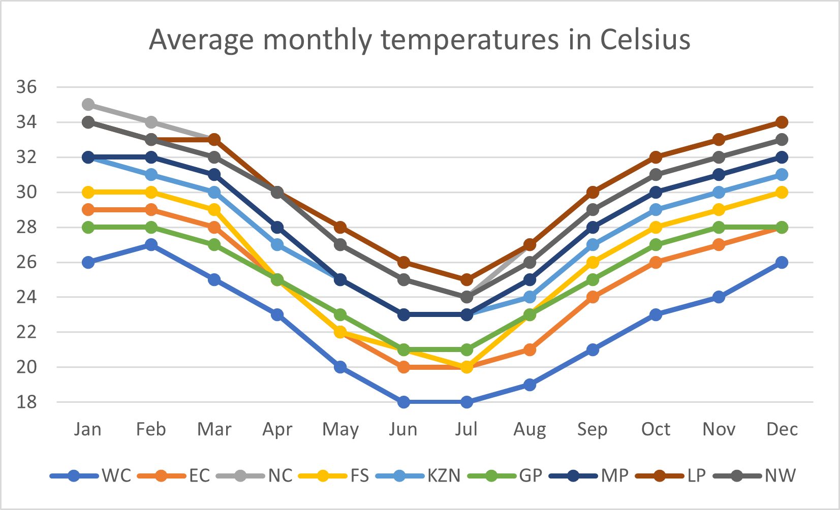
Figure 2.7: Figure 7: Time series of monthly maximum temperature per province
2.2.2.4.3 Image data
Image data is popular in the field of computer vision and AI. Images are typically represented as a set of three matrices, or grids, representing the red, blue and green values of each pixel in the image.
Figures @(fig8) and @(fig9) show an example of an image, and its decomposition into its red, green and blue components.

Figure 2.8: Example of image data (Photo by Andrew S on Unsplash)

Figure 2.9: An image split into its red, green and blue components
Images can also consist of more grids. Satellite images, for example, typically have additional grids with infrared values, water and vegetation indices, etc. These can be used to measure the presence of vegetation, water, and buildings, assess the health of vegetation, monitor climate change, and much more.
2.2.2.4.4 Spatial data
Spatial data is concerned with the locations of phenomena. Spatial data can include satellite images, GPS locations, GPS routes, and more. Figure 10 shows an example of a satellite image of central Pretoria, as well as GPS locations of some points of interest, and lines representing the roads. These are all examples of spatial data.
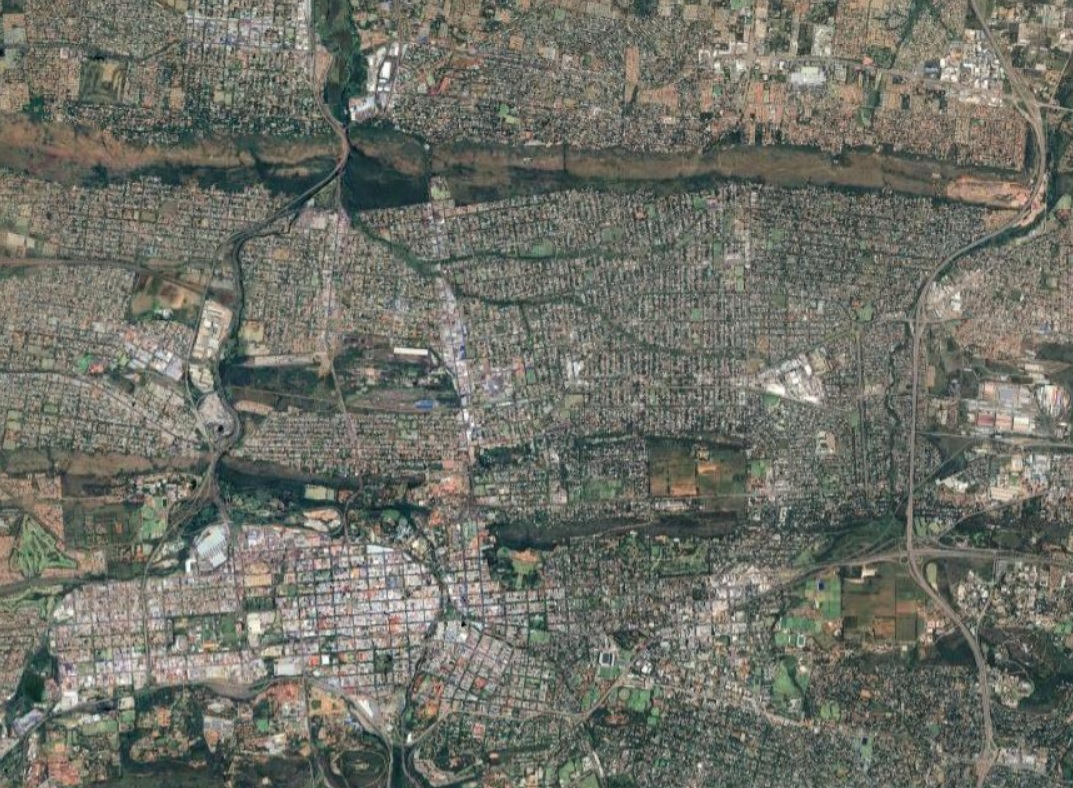
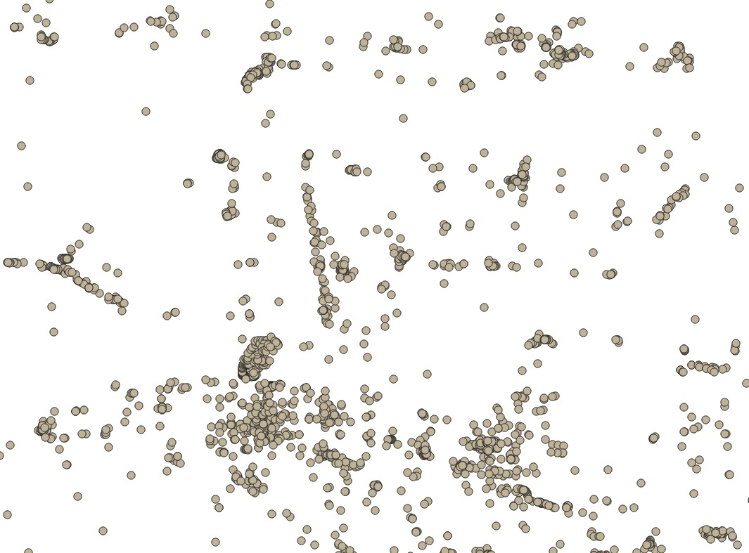
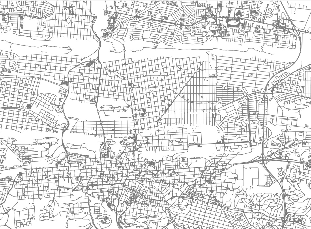
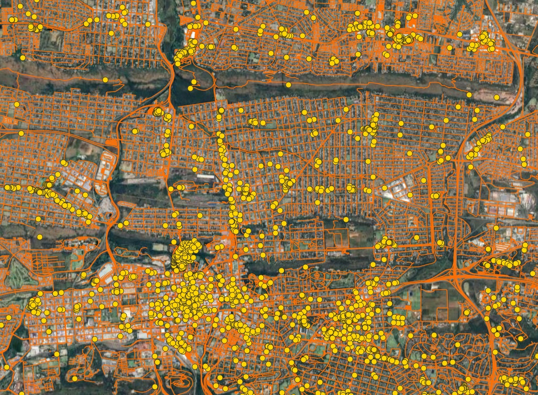
Figure 2.10: Top left: A satellite image; Top right: points of interest; Bottom left: roads; Bottom right: All previous datasets overlaid
Spatial data is used in urban planning, ecology, epidemiology (the study of disease spread), and more.
2.2.2.4.5 Audio data
Audio data can be found in sound files. This can include, among other things, music, audio tracks for movies, and voice recordings (like voice notes). Audio data is represented by a time series signal where the amplitude of the sound wave is sampled at regular intervals. Figure @(fig:fig11) shows an example of an audio file.
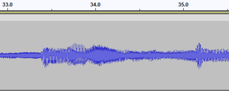
Figure 2.11: An audio file represented as a time series of amplitudes. Higher amplitudes represent a louder volume.
2.2.3 Structured and Unstructured data
Data can also be categorized into two types: Structured and Unstructured data. Structured data is organized and has a fixed format that makes it easy to work with. It typically follows a predefined scheme such as a table with rows and columns as with the data shown in Figure 2.1. Some other examples of structured data include spreadsheets (e.g. Excel) and Comma Separated Values (CSV) files. Unstructured data do not have a predefined format making them more challenging to work with. They includes data such as text (e.g. emails), images, videos, audio and other forms of data which cannot be stored using tables.
2.2.4 Data Types and Computers
The last part of this chapter considers how data of different types are stored on computers. We will look at the possible values that the data can be stored as, and common file extensions for each data type.
2.2.4.1 Qualitative data
Qualitative data is stored differently depending on whether it is nominal, ordinal, or text data (e.g. a response to an open-ended survey question).
- Nominal data: This is stored as labels, either text (for example, province codes like “GP”, “WC”, “LP”) or as integers representing categories (for example, 1 to represent Coastland and 2 to represent Inland in the Coastal (1) or Inland (2) variable in the Provinces dataset).
- Ordinal data: Stored in the same way as nominal data, but with an implied order.
- Text data: Stored as string variables, which is a standard data type on computers.
Qualitative data can be stored in text files (file extention: .txt) or in spreadsheets (file extention: .csv, .xlsx).
2.2.4.2 Quantitative data
- Discrete data: Stored as integers.
- Continuous data: Stored as real numbers, also called floating-point numbers. Ratio data and interval data can be stored this way.
Quantitative data is usually stored in spreadsheets (file extention: .csv, .xlsx).
2.2.4.3 Other data types
| Data type | Common file extensions |
| Time series | .csv, .xlsx |
| Image data | .png, .jpg, .bmp, .tiff |
| Spatial data | .shp, .json, .geojson |
| Audio data | .wav, .mp3 |
| Video data | .mkv, .avi, .mp4 |
2.2.4.4 Common data type mistakes
The previous sections explained how data of various types and scales of measurement should be stored. However, data can be stored in different ways, it can happen that data is stored incorrectly, or in a way that is unsuitable for use.
Exercise: Type a date in Excel, e.g. “10-10”. When you press Enter, it should automatically correct to a date (10 October). See what happens when you change the cell’s format to Text or Number. Now redo the exercise by first setting the format of the cell to text, and then typing in “10-10”. What happens now?
Key takeaway: The same data can be stored on a computer in a variety of ways. It is up to you, as the analyst, to understand how the data should be stored for your analysis.
2.2.5 Review
Give the data type (qualitative, quantitative discrete, quantitative continuous, or other) of the following variables and explain your answer.
- Province
- Coastal (1) or Inland (2)
- Population size
- HDI
- % of agricultural households
- Land area (sq km)
- Population density (per sq km)
- % of households with no internet access
- Sex ratio
- Median age
- Summer temp
- Province where most of the population migrate
If you are struggling to identify the data type of a variable, ask yourself the following questions:
- Does the variable have numerical values?
- If so, can you perform meaningful mathematical operations on the values, or are they just category labels?
- If so, do the values have to be whole numbers (e.g., number of people), or does it make sense for them to have decimals (e.g. percentages)?
Bonus question: Consider the variables Longitude and Latitude in the Provinces dataset. What kind of data do you think these variables are? What if you consider them together?