Chapter 2 Introduction to Probability

Now that you have learned about data, how to collect it and summarise it, you are now ready to make use of the sample data to draw meaningful conclusions about the sampled population. This process is referred to as inferential statistics and the essential statistical tool involved in this process is called probability. At its core, probability is a measure of our uncertainty. Everyday we are faced with decision-making and probability statements. Statements involving words such as chance, likelihood, odds, likely, expected, possibility and probably are all addressing the same issue: uncertainty. Every day we say, read or hear statements such as the following:

There is a 75% chance of rain today.
What is the likelihood we will a test today?
I will probably pass this course.
The odds are 1 in 100 million that you will be struck by lightning.
If a single fair coin is tossed, there is a 50-50 possibility that a head will occur.

In statistics, probability allows you to evaluate the reliability of your conclusions about the population when you have only information from the sample data. Consider the example 5. of tossing a coin once, the outcome will be either a head (H) or a tail (T). Suppose, as is true in reality, that you don’t know whether or not the coin is fair. You decide to perform a simple experiment by tossing the coin \(n=10\) times and observe \(10\) heads in a row. Can you conclude that the coin is fair? Probably not, because a fair coin is very unlikely to yield \(10\) heads in a row. It is more likely that the coin is biased.

As with the coin-tossing example, in statistics we use probability in two ways. When the population is known (e.g. the coin is known to be fair), probability is used to describe the chance of observing a particular sample outcome. When the population is unknown (e.g. it is unknown whether or not the coin is fair) and only a sample from the population is available, probability is used to make statements about the population. The latter case is more likely in practice. This is the inferential statistics we referred to above.

You know have an intuitive feeling for probability. In this chapter, we build on this intuition by presenting the basic mathematical concepts of probability along with some real-world examples.

2.1 Sample space and events

2.1.1 Sample space

We introduce the concept of an experiment as any action or process that results in well-defined observations or outcomes. On any single repetition or trial of an experiment, one and only one possible outcome will occur. The following are examples of experiments and their possible outcomes:

Experiment: Observing the gender of a new born baby; Outcomes: Male, Female
Experiment: Toss a coin; Outcomes: Head, Tail
Experiment: Selecting a part for inspection; Outcomes: Defective, Non-defective
Experiment: Conducting a sales call; Outcomes: Purchase, No-Purchase
Experiment: Rolling a die; Outcomes: 1,2,3,4,5,6
Experiment: Play a football game; Outcomes: Win, Lose, Tie

The outcomes of most experiments are uncertain. A set or collection of all possible outcomes of an experiment is called a sample space and it is denoted by \(S\).
The simplest experiment is one that has only two possible outcomes. Consider the first experiment above of observing the gender of a new born baby. The sample space for this experiment is given by \(S=\{M,F\}\), where \(M\) represents male and \(F\) represents female. Suppose that we observed the births of two new born babies, then the sample space is given by \(S_1=\{MM,MF,FM,FF\}\), where, for instance, \(MF\) indicates that the first baby born was male and the second baby born was female. Another possible sample space for this experiment might consist of the number of possible male births, \(S_2=\{0,1,2\}\). As a last example, consider the experiment of rolling a six-sided die, here the sample space is given by \(S_1=\{1,2,3,4,5,6\}\). Another sample space for this experiment might consist of whether the number facing up is even or odd, \(S_2=\{E,O\}\), where \(E\) represents an even number and \(O\) represents an odd number.

Example 2.1 Give the sample space for each of the following experiments.

Toss a coin first followed by a six-sided die.
Toss a coin until a tail occurs
Toss a R2 coin, R1 coin and R5 coin in that order
A piece of metal is measured to determine what fraction of it is gold.

Solutions

\(S=\{H1,H2,H3,H4,H5,H6,T1,T2,T3,T4,T5,T6\}\)
\(S=\{H,TH,TTH,TTTH,TTTTH,\dots\}\)
\(S=\{HHH,HTT,HHT,HTH,THT,TTH,THH,TTT\}\)
\(S=\{p|0<p<1\}\), where \(p=\) the proportion of the piece of metal that is gold

2.1.2 Events

In the study of probability, we are often interested in determining the likelihood of the occurrence of a collection of outcomes instead of the likelihood of the occurrence of a single outcome. For instance, in an experiment where three coins are tossed once, we might be interested in the outcomes which indicate that at least two heads are observed. This collection of outcomes denoted by \(A\), \(A={HHT,HTH,THH,HHH}\), is called an event. An event is any collection or subset of the sample space. An event is said to be simple if it consists of exactly one outcome and compound if it consists of more than one outcome. When an experiment is performed, a particular event, say \(A\), is said to occur if the resulting outcome is contained in \(A\).

Consider the experiment of tossing a R5 coin followed by a R1 coin. A sample space for this experiment could be \(S=\{HH,HT,TH,HH\}\). Some possible events are

\[ \begin{equation} E_1=\{HH\}\hspace{1cm}E_4=\{HH,TT\}\\ E_2=\{HT\}\hspace{1cm}E_5=\{HT,TH\}\\ E_3=\{TH\}\hspace{1cm}E_6=\{TT\} \end{equation} \] Events \(E_1\), \(E_2\), \(E_3\) and \(E_6\) are simple events and events \(E_4\) and \(E_5\) are compound events. There are actually a total of 16 possible events for the above experiment. As an exercise, identify the other events. Note that the empty set \(\emptyset\) and the sample space \(S\) are also events. The event \(\mathbf{E_1}\) can be described as getting a tail on the R5 and a tail on the R1. The event \(E_4\) can be described as getting two heads or two tails. As an exercise, describe the remaining events.

Example 2.2 Suppose an experiment consists of randomly selecting the exam scripts of three students. Each student’s script can either show a pass (P) or fail (F). The experiment has eight possible outcomes: \(FPP\), \(FPF\), \(FFP\), \(FFF\), \(PFF\), \(PFP\), \(PPF\) and \(FFF\). List the outcomes that correspond to each of the following events:

The first student failed
The first and last student failed
All the students passed
At least one student failed
At most one student failed

Solutions

\(E_1= \{FPP, FPF, FFP, FFF\}\)
\(E_2= \{FFF, FPF\}\)
\(E_3 = \{PPP\}\)
Note that at least one means one or more:

\[E_4=\{PFF, PFP, PPF, FPP, FPF, FFP, FFF\}\]

Note that at most one means one or less:

\[E_5 =\{PFP, PPF, PPP, FPP\}\]

Example 2.3 Consider the experiment of tossing a red six-sided die and a black six-sided die. This experiment consists of 36 possible outcomes. The sample space is given below:

\[\begin{matrix} (1,1)&(1,2)&(1,3)&(1,4)&(1,5)&(1,6)\\ (2,1)&(2,2)&(2,3)&(2,4)&(2,5)&(2,6)\\ (3,1)&(3,2)&(3,3)&(3,4)&(3,5)&(3,6)\\ (4,1)&(4,2)&(4,3)&(4,4)&(4,5)&(4,6)\\ (5,1)&(5,2)&(5,3)&(5,4)&(5,5)&(5,6)\\ (6,1)&(6,2)&(6,3)&(6,4)&(6,5)&(6,6) \end{matrix}\]

The first entry gives the outcome of the red die and the second entry gives the outcome of the black die. Thus, the outcome \((2,4)\), for instance, shows that the red die came up \(2\) and the black die came up \(4\).
Give the description of the following events:

\(\{(1,1),(2,1),(3,1),(4,1),(5,1),(6,1)\}\)
\(\{(1,1),(2,2),(3,3),(4,4),(5,5),(6,6)\}\)
\(\{(3,4),(4,3),(5,2),(2,5),(6,1),(1,6)\}\)
\(\{(5,6),(6,5)\}\)
\(\{(1,1)\}\)

Solutions

The black die shows 1
The two die match
The sum of the dice equals 7
The sum of the dice equals 11
Both dice show a 1

Example 2.4 For the dice-tossing experiment in Example ?? list the outcomes for the following events:

The sum is even.
The sum is divisible by 5.
The sum is a prime number. (A prime number is a number greater than 1 which is divisible only by 1 and itself.)
The number on the black die is 2 greater than the number on the red die.
The sum is not even.
The sum is not exactly divisible by 5

Solutions

The following pairs have a sum that is even:

\[\begin{matrix} (1, 1)&(1, 3)&(1,5)&(2, 2)&(2, 4)&(2, 6)\\ (3, 1)&(3, 3)&(3, 5)&(4, 2)&(4,4)&(4, 6)\\ (5, 1)&(5, 3)&(5, 5)&(6, 2)&(6,4)&(6, 6) \end{matrix}\]

The following pairs have a sum that is divisible by 5:

\[\{(1,4),(4, 1),(3,2),(2, 3),(5, 5),(6,4),(4, 6)\}\]
The following pairs have a sum that is a prime number:

\[\begin{matrix} (1,2)&(2, 1)&(1,4)&(4, 1)&(1,6)&(6, 1)&(2, 5)\\ (5, 2)&(3,4)&(4, 3)&(5, 6)&(6, 5)&(2, 3)&(3,2) \end{matrix}\]

The following pairs have a number on the black die that is 2 greater than the number on the red die:

\[\{(1,3),(2,4),(3,5),(4,6)\}\]
All outcomes in \(S\) that are not listed in part (a) have a sum that is not even.
All outcomes in \(S\) that are not listed in part (b) have a sum that is not divisible by 5.

Exercises

A single die is tossed. List the simple events in the sample space and the list the simple events in
1. \(A:\) Observe a number that is divisible by \(3\)
2. \(B:\) Observe a number less than \(5\)
3. \(C:\) Observe a number greater than \(2\)
A sample space contains seven simple events: \(E_1,E_2,\dots,E_7\). Use the following three events - \(A=\{E_3,E_4,E_6\}\), \(B=\{E_1,E_3,E_5,E_7\}\), and \(C=\{E_2,E_4\}\) and list the simple events in
1. Both \(A\) and \(B\)
2. Not \(A\)
3. \(A\) or \(C\) or both
For each of the following experiments, define the simple events.
1. A coin is tossed twice and the upper face (head or tail) is recorded for each toss.
2. Three children are randomly selected and their gender is recorded
Let \(C\) be the event that tomorrow’s weather is hot, and \(D\) the event that it rains tomorrow. Describe (in words) the following compound events
1. \(C\) or \(D\)
2. \(C\) and \(D\)
An experiment consists of asking three shoppers at random if they buy brand A peanut butter. Let \(Y\) denote yes and \(N\) denote no. Let \(YYN\) denote the simple event that the first two polled buy brand A and the third does not. Further, let \(E\) be the event that at least two people say yes and let \(F\) be the event that the first person polled say no. List the simple events making up the following events:
1. \(E\)
2. \(F\)
3. \(E\) or \(F\)
4. \(E\) and \(F\)

2.2 Some relationships between events

An event is nothing but a set. Therefore, relationships and results from set theory can be used to study events. The following operations will be used to construct new events from given events:

The union of two events \(A\) and \(B\), denoted by \(A\cup B\) and read “A or B” is the event consisting of all outcomes that are either in \(A\) or in \(B\) or in both events. This implies that the union includes outcomes for which both \(A\) and \(B\) occur as well as outcomes for which exactly one occurs. That is, all outcomes in at least one of the events.
The intersection of two events \(A\) and \(B\), denoted by \(A\cap B\) and read “A and B” is the event consisting of all outcomes that are in both \(A\) and \(B\).
The complement of an event \(A\), denoted by \(A^c\), is the set of all outcomes in \(S\) that are not contained in \(A\).

Example 2.5 Consider the experiment of rolling a balanced six-sided die.

Let \(A=\{1,3,5\}\), \(B=\{2,4,6\}\) and \(C=\{1,2,3\}\). Then

\(A\cup B=\{1,2,3,4,5,6\}=S\), \(A\cup C=\{1,2,3,5\}\), \(A\cap C=\{1,3\}\) and \(A^c=\{2,4,6\}\)

Sometimes \(A\) and \(B\) have no outcomes in common, so that their intersection contains no outcomes.

If events \(A\) and \(B\) have no outcomes in common, they are said to be disjoint or mutually exclusive events. This can be expressed mathematically as \(A\cap B=\emptyset\), where \(\emptyset\) denotes the event consisting of no outcomes whatsoever (the “null” or “empty” event).

Example 2.6 (Example 2.5 Continued) The events \(A\) and \(B\) are mutually exclusive because \(A\cap B=\emptyset\).

Example 2.7 Consider the experiment of tossing a R5 coin followed by a R1 coin. Are the following events mutually exclusive?

\(A=\) two heads; \(B=\) two tails
\(A=\{HT,TT\}\); \(B=\{HT,TH\}\)
\(A=\emptyset\); \(B=\{TT\}\)
\(A\); \(A^c\)

Solutions

Yes; they have no outcomes in common
No; they have the event \(HT\) in common
Yes; they have no outcomes in common
Yes; they have no outcomes in common

Sometimes it helps to use a picture called a Venn diagram to describe an experiment. A Venn diagram is a graphical representation of the sample spaces and the relationships between the events. A rectangle commonly denotes the sample space and the events are represented by circles drawn inside the rectangle. Figure 2.1 shows examples of Venn diagrams

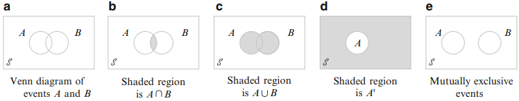
Figure 2.1: Venn diagrams

Exercises

Cumesh and Fani have applied for several part-time student jobs at a local university. Let \(A\) be the event that Cumesh is hired and let \(B\) be the event that Fani is hired. Express in terms of \(A\) and \(B\) the events

Cumesh is hired but not Fani
At least one of the is hired
Excactly one of them is hired

An academic department has just completed voting by secret ballot for a department head. The ballot box contains four slips with votes for candidate \(B\) and three with votes for candidate \(A\). Suppose these slips are removed from the box one by one.

List all the possible outcomes
Suppose a running tally is kept as slips are removed. For what outcomes does \(A\) remain ahead of \(B\) throughout the tally.

Which of the following pairs of events are mutually exclusive?

\(E=\) Mrs. Botha gives birth to twins. \(F=\) A mother gives birth to a girl
\(E=\) Lebogang fails the last Statistics test \(F=\) Lebogang passes the course
\(E=\) Kwanele goes to the movies \(F=\) Kwanele eats pop-corn

A student is currently working on three assignments for three different subjects. Let \(A_i\) denote the event that the \(i^{th}\) assignment is completed by the due date. Use the operations of union, intersection, and complement to describe each of the following events in terms of \(A_1\), \(A_2\), and \(A_3\), draw a Venn diagram, and shade the region corresponding to each one.

At least one assignment is completed by the due date.
All the assignments are completed by the due date.
Only the first assignment is completed by the due date.
Exactly one assignment is completed by the due date.

2.3 Assigning Probabilities

2.3.1 What is a probability?

To every event \(E\) in the sample space \(S\), we assign a number \(P(E)\) called the probability of \(E\). The probability of an event is a number between \(0\) and \(1\). It is the likelihood that the event \(E\) will occur. The closer \(P(E)\) is to \(1\), the more likely the event \(E\) is to occur. The closer \(P(E)\) is to \(0\), the more unlikely the event \(E\) is to occur. Probability satisfies the following properties:

\(0<P(E)<1\)
\(P(S)=1\)
If \(E_1,E_2,E_3,\dots\) form sequences of pairwise mutually exclusive events of \(S\), that is \(E_i\cap E_j=\emptyset\), for \(i\neq j\), then \(P(E_1\cup E_2\cup E_3\cup\dots)=\sum_{i}P(E_i)\)

where \(\sum_{i}P(E_i)\) is the sum of the probabilities of all the outcomes in a sample space. Consider a compound event \(A\). The probability of \(A\) is defined to be the sum of the probabilities of the outcomes contained in \(A\).

Example 2.8 Suppose a six-sided die is tossed once and the probability of any side landing face up is \(\frac{1}{6}\). If \(E\) is the event of getting an even number and \(F\) is the event of getting an odd number, find

\(P(E)\)
\(P(F)\)
\(P(E~\text{or}~F)\)
\(P(E~\text{and}~F)\)

Solutions

The sample space is \(S=\{1,2,3,4,5\}\), the event \(E\) is \(\{2,4,6\}\), and the event \(F\) is \(\{1,3,5\}\). We thus have:

\(P(E)=P(2)+P(4)+P(6)=\frac{1}6+\frac{1}{6}+\frac{1}{6}\)
\(P(E)=P(1)+P(3)+P(5)=\frac{1}6+\frac{1}{6}+\frac{1}{6}\)
\(P(E~or~F)=P(E\cup F)=P(S)=1\)
\(P(E~and~F)=P(E\cap F)=0\), because \(E\cap F=\emptyset\).

We next turn to the main question of this section which is on how to assign probabilities to events. There are three approaches for assigning probabilities to events: the objective approach, the classical approach and the subjective approach. On the other hand We now discuss each method in turn.

2.3.2 Objective approach

The objective approach involves assigning probabilities to events based on the proportion of times that events of the same kind will occur in the long run. Consider an experiment that can be repeatedly performed in an identical and independent fashion and let \(A\) be an event consisting of a fixed set of outcomes of the experiment. Simple examples of repeatable experiments include tossing a coin and rolling a die. If the experiment is performed \(n\) times, on some of the replications the event \(A\) will occur and on some \(A\) will not occur. Let \(n(A)\) denote the number of replications on which \(A\) does occur. Then the ratio \(n(A)/n\) is called the relative frequency of occurrence of the event \(A\) in the \(n\) replications. The empirical evidence based on the results of many of the sequences of repeatable experiments indicate that as \(n\) becomes large, the relative frequency stabilizes. That is, as \(n\) gets large, the relative frequency approaches a limiting value referred to as the limiting relative frequency of the event \(A\). The objective method of assigning probability identifies this limiting relative frequency with \(P(A)\). Thus, if an experiment is repeatable, we can assign probabilities to the outcomes in accordance with their limiting relative frequencies. As an example, The table below contains the number of heads obtained when a fair coin was tossed \(n\) times, as well as the relative frequency \(n(H)/n\) for the number of heads obtained in each case. It is clear from the table that the limiting value of the relative frequency of obtaining a head when a coin is tossed \(n\) times will approach \(0.5\) as \(n\) becomes large. Therefore, the probability of \(H\), obtaining a head, is \(0.5\).

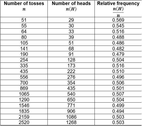
The only problem with this approach is that the limiting relative frequencies of events are not always known. In order to use this method, we need to have repetitive data available and then use it to approximate the relative frequency limits. Probabilities obtained using this approach are said to be empirical. According to the empirical approach to probability, if \(A\) is an event, \(P(A)\) is approximately equal to \(f/n\), where \(f\) is the number of favorable outcomes and \(n\) is the number of repetitions of the experiment. Thus, \(P(A)\approx f/n\). For example, consider again the coin-tossing experiment. The relative frequency can serve as an estimate of the probability \(P(H)\). To get a better estimate, we could consider tossing the coin \(3000\) or \(5000\) times or even more.

Example 2.9 The NBT math scores for 18790 students at a large university are given in the following grouped frequency table:

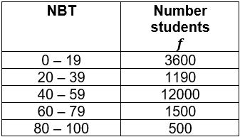
Figure 2.2: Tree diagram for the experiment of tossing two coins

If a student is selected at random, what is the probability that the student’s NBT math score

exceeds 39
is at most 59
is between 60 - 79

Solutions We first calculate the relative frequencies for each class by dividing the frequency \(f\) of the class by the total number of students \(n=18790\).

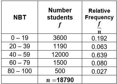
Figure 2.3: Tree diagram for the experiment of tossing two coins

\(P(NBT>39)=0.343+0.157+0.043+0.014=0.557\)
\(P(N\leq 59)=0.103+0.340+0.343+0.157=0.943\)
\(P(60<NBT<79)=0.043\)

2.3.3 Classical approach

The classical approach to assigning probabilities considers the case when all the outcomes are equally likely to occur. Consider an experiment with a finite number, \(n\), of outcomes that we believe are equally likely to occur. We can assign each outcome in the sample space \(S\) a probability value of \(1/n\). This is a consequence of the second property of a probability, which states that the sum of the probabilities for a sample space must be \(1\). Then if \(E\) is an event containing \(n(E)\) outcomes, the probability of \(E\) occurring is simply \(n(E)/n\). Thus, we have the following basic fact:

*If \(S\) is a sample space of equally likely outcomes, then \(P(E)=n(E)/n\),

where \(n(E)\) is the number of outcomes in \(E\) and \(n\) is the number of outcomes in \(S\).

The objective method for assigning probabilities using sample spaces of equally likely outcomes is referred to as the classical probability method.

Example 2.10 Consider the dice-tossing experiment described in Example 2.3. Find the probability that

Both dice show an even number.
The dice show a sum of \(7\)
The dice show a sum of \(7\) or \(11\)
Both dice show a prime number
The dice show a sum of \(13\)

Solutions

Recall that the sample space is \[\begin{matrix} (1,1)&(1,2)&(1,3)&(1,4)&(1,5)&(1,6)\\ (2,1)&(2,2)&(2,3)&(2,4)&(2,5)&(2,6)\\ (3,1)&(3,2)&(3,3)&(3,4)&(3,5)&(3,6)\\ (4,1)&(4,2)&(4,3)&(4,4)&(4,5)&(4,6)\\ (5,1)&(5,2)&(5,3)&(5,4)&(5,5)&(5,6)\\ (6,1)&(6,2)&(6,3)&(6,4)&(6,5)&(6,6) \end{matrix}\] Therefore, there are \(n=36\) equally likely outcomes.

Let \(E_1\) be the event that both dice show an even number. There are \(n(E_1)=9\) outcomes in which both numbers are even. Therefore, \(P(E_1)=n(E_1)/n=9/36=1/12\).
Let \(E_2\) be the event that the dice show a sum of \(7\). \(E_2=\{(3,4);(4,3);(5,2);(2,5);(6,1);(1,6)\}\). Therefore, \(P(E_2)=n(E_2)/n=6/36=1/6\)
Let \(E_3\) be the event that the dice show a sum of \(7\) or \(11\). \(E_3=\{(3,4);(4,3);(5,2);(2,5);(6,1);(1,6);(5,6);(6,5)\}\). Therefore, \(P(E_3)=n(E_3)/n=8/36=2/9\).
Let \(E_4\) be the event that both dice show a prime number. Since \(E_4=\{(2,2);(2,3);(2,5);(3,2);(3,5);(5,2);(5,3);(5,5)\}\), we have \(P(E_4)=n(E_4)/n=8/36=2/9\).
Let \(E_5\) be the event that the two dice show a sum of \(13\). Since a sum of \(13\) is impossible, \(E_6=\emptyset\). Thus, \(P(E_6)=0\).

2.3.4 Subjective approach

The objective method of assigning probabilities is limited to experimental situations that are repeatable. However, many real-world experimental situations are unrepeatable. For instance, the chances of a peace agreement in the Russia-Ukraine war. Thus, we have limited or no information concerning the outcomes of an experiment. We must therefore adopt an alternative interpretation of a probability. In such situations, probabilities are assigned based on experience or expert knowledge. For instance, a doctor treating a patient with a rare disease must make a prognosis based on his experience with the patient and the patient’s overall medical record. When probabilities are assigned to events based on intuition and personal beliefs, the assignment method is called subjective. Because different people may have different prior information and opinions concerning a given experimental situation, probability assignment will differ from individual to individual.

Exercises

Match each of the following probabilities with one of the statements that follow:

\[ 0\quad 0.01\quad 0.3\quad 0.99\quad 1\]

The event is very unlikely, but it will occur once in a while in a long sequence of trials.
The event will occur more often than not.
The event is certain.
The event is impossible. It can never happen.

Which of the following numbers cannot be the probability of some event?

\(0.74\)
\(-1\)
\(1.02\)
\(0.67\)

A 2024 survey showed that of the top 10 electric vehicles based on cost, 2 are BYDs, 2 are Toyotas, 3 are Renaults and 3 are Volvos. Choose one at random. What is the probability that the chosen EV is

Asian?
European?
Asian or European?

A bag contains three red pens, two blue pens and five black pens. One pen is selected at random. What is the probability that the pen is

red?
blue?
black?

Suppose that two dice are rolled one time, what is the probability of getting

a sum of 6?
doubles?
a sum of 7 or 11?
a sum greater than 9?

In a study concerning the distribution of the ages of female CEOs in South Africa, 1 CEO was found to be aged between 21 - 30, 8 CEOs were between 31 - 40, 27 CEOs were between 41 - 50, 29 CEOs were between 51 - 60, 24 CEO were between 61 - 70 and 11 CEOs were 71 years or older. Suppose that a CEO is selected at random , what is the probability that her age is

between 31 and 40?
under 31?
over 30 and under 51?
under 31 or over 60?

Toss three coins 128 times and record the number of heads (0, 1, 2, or 3); then record your results with the theoretical probabilities. Compute the empirical probabilities of each.

2.4 Mathematical properties of probability

We now mention some other important and useful mathematical properties of probabilities.

2.4.1 Probability of a complement

If events \(A\) and \(A^c\) are complementary events in the sample space \(S\), then \(P(A^c)+P(A)=1\). Solving for \(P(A^c)\), we obtain \(P(A^c)=1-P(A)\). As an example, suppose that the probability that Loyiso will finish his assignment before the deadline is \(\frac{3}{7}\). What is the probability that he will not finish his assignment? Let \(A\) be the event that Loyiso will finish his assignment. Then, \(A^c\) is the event that he will not finish his assignment. Since \(P(A)=\frac{3}{7}\), we have \(P(A^c)=1-P(A)=1-\frac{3}{7}\).

2.4.2 Addition rule

For any events \(A\) and \(B\), \(P(A\cup B)=P(A)+P(B)-P(A\cap B)\). This is known as the addition rule. This rule is useful when we are interested in knowing the probability that at least one of two events occurs. That is, with events \(A\) and \(B\), we are interested in knowing the probability that event \(A\) or event \(B\) or both will occur.

Example 2.11 In a certain residential suburb, \(60\%\) of all households get internet service from the local cable company, \(80\%\) get television service from that company, and \(50\%\) get both services from the company. If a household is randomly selected, what is the probability that it gets at least one of these services from the company?

Solution: Let \(A=\) the event that a household gets internet service from the cable company and \(B=\) the event that household gets television service from the cable company. The given information implies that \(P(A)=0.6\), \(P(B)=0.8\) and \(P(A\cap B)=0.5\). \(P(\text{at least one of the services from the company})=P(A)+P(B)-P(A\cap B)=0.6+0.8-0.5=0.9\).

Exercises

Consider randomly selecting a student at a certain university, and let \(A\) denote the event that the selected student uses ChatGPT and \(B\) be the event that the student uses deepseek. Suppose that \(P(A)=0.5\), \(P(B)=0.4\) and \(P(A\cap B)=0.25\).

Calculate the probability that the selected student uses at least one of the two chatbots (i.e. the probability of the event \(P(A\cup B)\)).
What is the probability that the selected student uses neither of the two chatbots?
Describe, in terms of \(A\) and \(B\), the event that the selected student uses ChatGPT but not deepseek and then calculate the probability of this event.

A particular University has elected both the president and deputy president of the student representative council. Let \(A\) be the event that a randomly selected voter favors the presidential candidate and \(B\) be the event that the voter favors the deputy presidential candidate. Suppose that \(P(A^c)=0.44\), \(P(B^c)=0.57\) and \(P(A\cup B)=0.68\).

What is the probability that a randomly selected voter is in favor of both candidates?
What is the probability that a randomly selected voter is in favor of exactly one of these
candidates?
What is the probability that a randomly selected voter is not in favor of at least one of these candidates?

A student has three options on what to do for leisure. Let \(A_i=\{\text{do activity } i\}\), for \(i=1,2,3\), and suppose that \(P(A_1)=0.22\), \(P(A_2)=0.25\), \(P(A_3)=0.28\), \(P(A_1\cap A_2)=0.11\), \(P(A_1\cap A_3)=0.05\), \(P(A_2\cap A_3)=0.07\). Express in words each of the following events and compute the probability of each event::

\(A_1\cup A_2\)
\(A_1^c\cap A_2^c\) [Hint: \((A_1\cup A_2)^c=A_1^c\cap A_2^c\)]

Let \(A\) be the event that the next customer that walks into a store will buy Coke and let \(B\) be the event that the next customer that walks into a store will buy Pepsi. Suppose that \(P(A)=0.3\) and \(P(B)=0.5\).

Why is it not the case that \(P(A)+P(B)=1\)?
Calculate \(P(A^c)\).
Calculate \(P(A\cup B)\).
Calculate \(P(A^c\cap B^c)\). [Hint: Use the hint in the previous question]

2.5 Basic counting rules

Whenever the outcomes of an experiment are equally likely (that is, the same probability is assigned to each simple event in the sample space), a necessary step towards assigning probabilities is being able to count. Suppose that an experiment has \(n\) possible outcomes and \(n(A)\) is the number of experimental outcomes contained in event \(A\), then \(P(A)=n(A)/n\). If all the experimental outcomes are available or can be listed, then \(n(A)\) and \(n\) can be obtained without the use of counting rules. However, many experiments involve constructing lists of outcomes in which \(n\) and \(n(A)\) are prohibitively large. Fortunately, for such experiments, we can use some basic counting rules to calculate probabilities without listing the experimental outcomes.

2.5.1 The Fundamental counting rule

The first counting rule we discuss is referred to the fundamental counting rule and it applies to experiments with multiple steps. Consider an experiment in which five coins are tossed. Let the experimental outcomes be defined in terms of the patterns of heads and tails appearing on the upward faces of each of the five coins. What is the total number of experimental outcomes? Let \(H\) and \(T\) denote a head and a tail, respectively, \((H,H,H,H,H)\) indicates the experimental outcome with a head on the first coin, second coin, third coin, fourth coin and fifth coin. As can be seen, it is a cumbersome task to list all of the experimental outcomes in the sample space \(S\). To help us calculate the total number of experimental outcomes without listing them, the experiment of tossing the five coins can be thought of as a five-step experiment: In the first step, the first coin is tossed; in the second step, the second coin is tossed; in the third step, the third coin is tossed; in the fourth step, the fourth coin is tossed and in the fifth step, the fifth coin is tossed. We can make use of the fundamental counting rule to determine the number of experimental outcomes.

Theorem 2.1 (Fundamental Counting Rule) If an experiment can be described as a sequence of \(k\) steps with \(n_1\) possible outcomes on the first step, \(n_2\) possible outcomes on the second step, and so on, then the total number of exeprimental outcomes is given by \(n_1\times n_2 \times \dots \times n_k\).

Looking at the experiment of tossing five coins as a sequence of first tossing one coin (\(n_1=2\)), followed by the second coin (\(n_2=2\)), followed by the third coin (\(n_3=2\)), followed by the fourth coin (\(n_4=2\)) and then the last coin (\(n_5=2\)), we can see from the fundamental counting rule that there are \(2\times 2\times 2\times 2\times 2=32\) experimental outcomes.

Example 2.12 Consider the experiment of going to a store to buy a new phone. Once there, you find you can select from 4 models each with 5 different battery options and a choice of 15 exterior colors. How many possible choices are there for you to make?

Solution: The experiment has three steps: The first step (Step 1) involves choosing one of the \(n_1=4\) models, the second step (Step 2) involves choosing one of the \(n_2=5\) battery options and the third step (Step 3) involves choosing one of the \(n_3=15\) exterior colors. Therefore, by the fundamental counting rule, there are \(n_1\times n_2\times n_3=4\times 5\times 15=300\) possible choices.

2.5.2 Tree Diagrams

In many counting and probability problems, a visual representation of all the outcomes of a multiple-step experiment can be constructed using a tree diagram. Suppose that, in the above coin-tossing experiment, we only tossed two coins. Figure 2.4 displays a tree diagram for the experiment of tossing two coins. The sequence of steps moves from the left to right. The first step (Step 1) involves tossing the first coin and the second step (Step 2) involves tossing the second coin. For each step, there are two possible outcomes: head (\(H\)) or tail (\(T\)). Note that each possible outcome in the first step is associated with two branches in the second step. The points (e.g. \((H,H)\)) on the right side of the tree corresponds to the experimental outcomes. Each path from the leftmost node of the tree to the rightmost node of the tree results in a single experimental outcome.

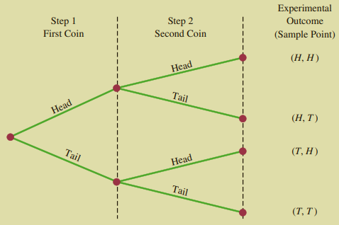
Figure 2.4: Tree diagram for the experiment of tossing two coins

2.5.3 Combinations

The second counting rule is useful when an experiment involves selecting a subset of \(k\) elements from a set of \(n\) distinct elements. The resulting sequence of \(k\) elements is called a combination. The number of combinations of size \(k\) from \(n\) distinct elements, denoted by \(C^n_k\), can be calculated as follows \[\begin{eqnarray} C^n_k&=&\binom{n}k\\ &=&\frac{n!}{k!(n-k)!} \end{eqnarray}\] Factorial notation: For any positive integer \(n\), \(n!\) is read “\(n\) factorial” and is defined by \(n!=n\times(n-1)\times(n-2)\times\dots\times1\) and \(0!=1\), by definition. For instance, \(4!=4\times3\times2\times1=24\).

Example 2.13 Suppose you have five books but you only have space for two books on your bookshelf. In how many ways can you select two books from the five books?

Solution: Given that \(n=5\) and \(k=2\), there are \(C^5_2=\binom{5}2=10\) possible choices.

2.5.4 Permutations

The third counting rule is useful when an experiment involves selecting a subset of \(k\) elements from a fixed set of \(n\) distinct elements in such a way that the order of selection is important. Thus, the same \(k\) elements selected in a different order are considered a different experimental outcome. The resulting ordered sequence of \(k\) elements is called a permutation. The number of permutations of size \(k\) from \(n\) distinct elements, denoted by \(P^n_k\), can be calculated using the fundamental counting rule. The first element can be chosen in \(n\) ways, the second in \((n-1)\) ways and the \(k^{th}\) element in \((n-(r-1))\) ways. Thus,

\(P^n_k=n(n-1)(n-2)\times\dots\times(n-k+2)(n-k+1)\)

Using the factorial notation, \(P^n_k=\frac{n(n-1)\times\dots\times(n-k+1)(n-k)(n-k-1)\times\dots\times(2)(1)}{(n-k)(n-k-1)\times\dots\times(2)(1)}\)

which becomes, \(P^n_k=\frac{n!}{(n-k)!}\)

Example 2.14 Suppose you have three books but you only have space for two books on your bookshelf. In how many ways can you select and arrange the two books.

Solution: Given that \(n=5\) and \(k=2\), there are \(P^5_2=\frac{5!}{(5-2)!}=20\) possible ways to select and arrange the two books.

A special case of the permutation counting rule is when \(n=k\). Then, \(P^n_n=n!\) gives the number of ways to arrange a set of \(n\) distinct elements.

Example 2.15 How many ways can \(5\) books be arranged on a bookshelf?

Solution:

This is similar to selecting \(k=5\) books from \(n=5\) and then arranging them on a bookshelf. Thus, there are \(P^5_5=5!=120\) ways of arranging the 5 books on a bookshelf.

Exercises

If you are taking a true/false test with 10 questions, in how many different ways can you fill in your answer sheet if you are guessing the answer of each question?
How many different houses can be built if a builder offers a choice of five basic plans, three roof styles and two exterior finishes?
In how many ways can seven of ten monkeys be arranged in a row for a biology experiment?
The student representative council has five candidates for president and two candidates for deputy president. Use a tree diagram to determine the number of ways the two offices can be filled.
Three balls are selected from a box containing 10 balls. The order of selection is not important. How many simple events are in the sample space?
The same car model can be purchased from five different dealerships. In how many ways can three dealerships be chosen from the five?
A smartphone is composed of five critical parts that can be assembled in any order. A test is to be conducted to determine the time necessary for each order of assembly. If each order is to be tested once, how many tests must be conducted?

2.6 Finding probabilities using the basic counting rules

The next examples demonstrate how to use the three basic counting rules to solve probability problems.

Example 2.16 Suppose that four coins are tossed, what is the probability of getting four heads? Solution Let \(A=\) the event that four heads are observed.

We first determine the number of outcomes from tossing the four coins. This is a multiple-step experiment involving four steps each having two outcomes. Thus, there are \(2\times2\times2\times2=16\) possible outcomes. Next, only one outcome will result in four heads \((H,H,H,H)\). Putting it all together, we have \(n=16\) and \(n(A)=1\), the probability of \(A\) is \(P(A)=n(A)/n=1/16=0.0625\).

Example 2.17 Suppose that four coins are tossed, what is the probability that the first two coins are heads?

Solution: Let \(B=\) the event that the first two coins are heads

From the previous example, we know that there are 16 possible outcomes. The event \(B\) will occur if the first two coins are heads and the last two coins can be either heads or tails. This is a multi-step experiment involving four steps in which the first two steps have 1 outcome and the last two steps have 2 outcomes. Thus, there are \(1\times1\times2\times2=4\) ways in which the event \(B\) can occur. Putting it all together, \(n=16\) and \(n(B)=4\), the probability of \(B\) is \(P(B)=n(B)/n=4/16=0.25\).

Example 2.18 Five manufactures produce a certain electronic device, whose quality varies from manufacturer to manufacturer. If you were to select three manufacturers at random, what is the probability that the selection would contain exactly two of the best three?

Solution The experiment consists of randomly selecting three manufacturers from a group of five, three of which are designated as “best” and two as “not best”. Let \(C=\) the event of selecting two of the “best” three manufacturers

We first determine the number of ways of selecting any three of the five manufacturers. Thus, \(n=5\) and \(k=3\), by the counting rule for combinations, there are \(C^5_3=\binom{5}3=10\) ways to choose three manufactures from the five. Next, we determine the number of ways of selecting exactly \(2\) manufactures from the best \(3\). Note that this outcome involves a two step experiment. In the first step we must select \(2\) manufactures from the “best” three and in the second step we must select \(1\) manufacturer from the two “not best” manufacturers. With \(n=3\) and \(k=2\), there are \(C^3_2=\binom{3}2=3\) ways of performing the first step. Lastly, with \(n=2\) and \(k=1\), there are \(C^2_1=\binom{2}1\) ways of performing the second step. Thus, \(3\times2=6\) ways of selecting \(2\) of the “best” \(3\) manufacturers. Putting it all together, \(n=10\) and \(n(C)=6\), the probability of \(C\) is \(P(C)=n(C)/n=6/10=0.6\).

Exercises

The student representative council (SRC) must select two members from five (2 male and 3 female) candidates to be the president and deputy president of the SRC.

In how many ways can the two candidate be chosen in such a way that the president is always a female and the deputy president is always male?
Suppose that all the candidates have an equal chance of being chosen, what is the probability that the president is female and the deputy president is male?

Four equally qualified runners, Naledi, Jacques, Kim and Yusuf, run a 100-meter print and the order of finish is recorded.

How many orders of finish are possible?
What is the probability that Yusuf wins the sprint?
What is the probability that Yusuf wins and Naledi places second?
What is the probability that Kim finishes last?

A drawer contains four pairs of black socks, five pairs of green socks and six pairs of white socks. Suppose that three pairs of socks are randomly selected.

What is the probability that exactly two pairs of the selected pairs of socks are white?
What is the probability that all three of the selected pairs of socks are of the same color?
What is the probability that one pair of each color is selected?

2.7 Conditional probabilities

Most of the time, the probability of an event is influenced by whether or not a related event has already occurred. The probability of an event \(A\) occurring when we know that event \(B\) has already occurred is called a conditional probability and it is written as \(P(A|B)\). We use the notation \(|\) to indicate that we are considering the probability of event \(A\) given the condition that event \(B\) has occurred. Hence, the notation \(P(A|B)\) reads “the probability of \(A\) given \(B\)”. As an illustration of the application of conditional probability, we consider a study that was undertaken at a certain university to determine what relationship, if any, exists between mathematics ability and interest in mathematics. The ability and interest for \(150\) students were determined with the results summarized in the following table:

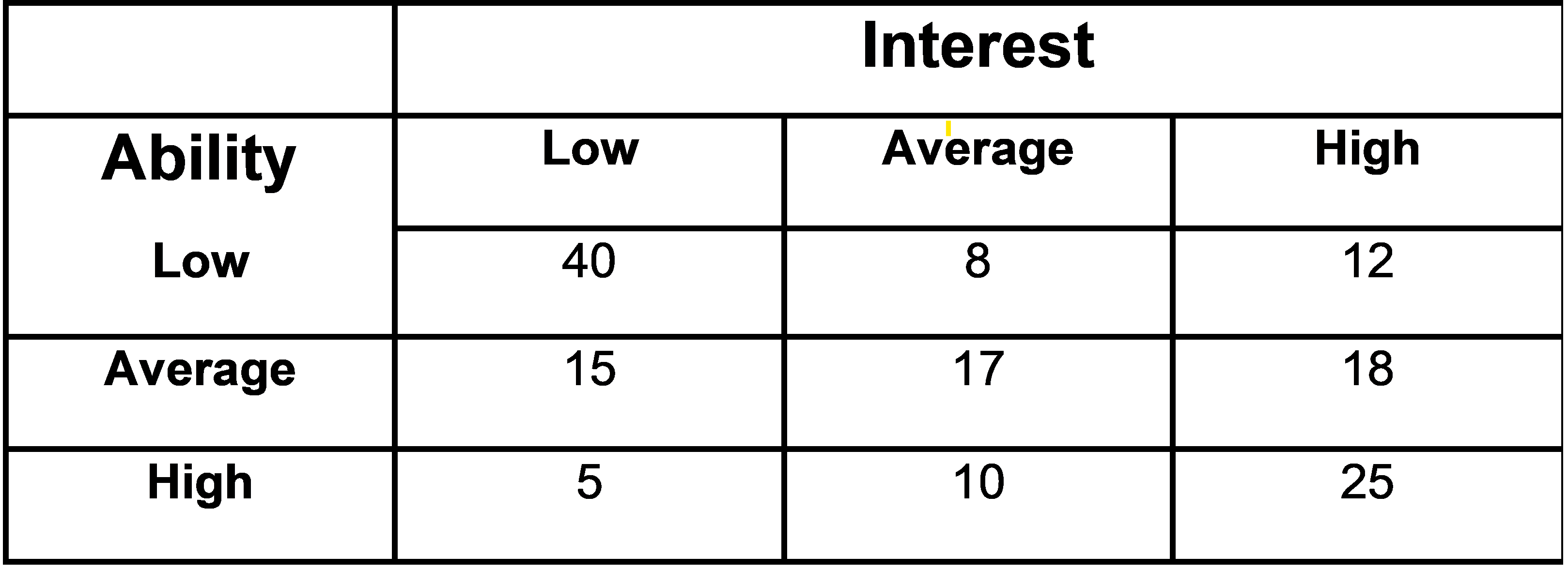
Let \(L_1=\) the event that a student has a Low interest in mathematics \(A_1=\) the event that a student has a Average interest in mathematics \(H_1=\) the event that a student has a High interest in mathematics \(L_2=\) the event that a student has a Low ability in mathematics \(A_2=\) the event that a student has a Average ability in mathematics \(H_2=\) the event that a student has a High ability in mathematics

Dividing the data values in the table by 150, we obtain \(P(L_1\cap L_2)=40/150=\), the probability that a student has a low interest and low ability in mathematics. \(P(L_1\cap A_2)=8/150=\), the probability that a student has a low interest and average ability in mathematics. \(P(L_1\cap H_2)=12/150=\), the probability that a student has a low interest and high ability in mathematics. \(P(A_1\cap L_2)=15/150=\), the probability that a student has an average interest and low ability in mathematics. \(P(A_1\cap A_2)=17/150=\), the probability that a student has a average interest and average ability in mathematics. \(P(A_1\cap H_2)=18/150=\), the probability that a student has an average interest and high ability in mathematics. \(P(H_1\cap L_2)=5/150=\), the probability that a student has a high interest and low ability in mathematics. \(P(H_1\cap A_2)=10/150=\), the probability that a student has a high interest and average ability in mathematics. \(P(H_1\cap H_2)=25/150=\), the probability that a student has a high interest and high ability in mathematics.

Since each of these values give the probabilities of the intersection of two events, the probabilities are called joint probabilities. Table ?? is referred to as the joint probability table. The table gives a summary of the probability information.

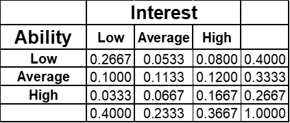
Figure 2.5: Joint probability table for the mathematics interest and ability study

The values in the margins of the joint probability table provide the probabilities of each event separately. That is, \(P(L_1)=0.4000\), \(P(A_1)=0.2333\), \(P(H_1)=0.3667\), \(P(L_2)=0.4000\), \(P(A_2)=0.3333\) and \(P(H_2)=0.2667\). These probabilities are referred to as marginal probabilities because of their location in the margins of the joint probability table. Note that the marginal probabilities are obtained by summing the joint probabilities in the corresponding row or column of the joint probability table. For example, the marginal probability of having a high ability in mathematics is \(P(H_1)=P(H_1\cap L2)+P(H_1\cap A2)+P(H_1\cap H2)=0.0333+0.0667+0.1667=0.2667\).\ We now turn to our initial task of assessing whether or not there is a relationship between mathematics ability and interest. We first calculate the conditional probability that a randomly selected student has a low ability in mathematics given that the student has a low interest in mathematics. In mathematical notation, we want to calculate \(P(L_2|L_1)\). Note that \(P(L_2|L_1)\) means that we are interested in the probability of \(L_2\) given that we only have \(L_1\) (that is, the student has a low interest in mathematics). Thus, \(P(L_2|L_1)\) means that we are only concerned with the mathematics ability of the \(60\) students who have a low interest in mathematics. Since \(40\) of the \(60\) students have a low mathematics ability, \(P(L_2|L_1)=40/60=2/3=0.6667\). Thus, given that a student has a low interest in mathematics, there is a \(67\%\) probability that the student has a low mathematics ability.\ We have shown that \(P(L_2|L_1)=40/60=0.6667\). Dividing both the numerator and denominator of this fraction by \(150\), the total number of students in the study, we get \[ \begin{aligned} P(L_2|L_1)=\frac{40}{60}=\frac{40/150}{60/150}=\frac{0.2667}{0.4000}=0.6667 \end{aligned} \] We can see that \(P(L_2|L_1)\) can be calculated as \(0.2667/0.4000\). Referring to the joint probability table (Table ??), we can see that \(0.2667\) is the probability \(P(L_1\cap L_2)\) and \(0.4000\) is the probability \(P(L_1)\). Therefore, \(P(L_2|L_1)\) can be expressed as a ratio of the joint probability \(P(L_1\cap L_2)\) to the marginal probability \(P(L_1)\)

\[ \begin{aligned} P(L_2|L_1)=\frac{P(L_1\cap L_2)}{P(L_1)}=\frac{0.2667}{0.4000}=0.6667 \end{aligned} \] This leads to the following general formula for calculating conditional probabilities. For any two events \(A\) and \(B\), \[ \begin{eqnarray} P(A|B)=\frac{P(A\cap B)}{P(B)}\\ \text{or}\\ P(B|A)=\frac{A\cap B}{P(A)} \end{eqnarray} \] The Venn diagram in Figure @(fig:fig8) illustrates concept of a conditional probability. The circle on the right shows that event \(B\) has occurred; the portion of the circle that overlaps with event \(A\) denotes the event \((A\cap B)\). We know that once event \(B\) has occurred, the only way that we can also observe event A is for the event \((A\cap B)\) to occur. Thus, the ratio \(P(A\cap B)/P(B)\) provides the conditional probability that we will observe event \(A\) given that event \(B\) has already occurred.

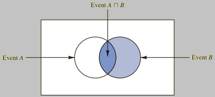
Figure 2.6: Motivating the definition of a conditional probability

2.7.1 Independent events

We now introduce the concept of independent events. Two events, \(A\) and \(B\) are said to be independent if \(P(A|B)=P(A)\), otherwise, they are said to be dependent. The idea behind the independence of events is that the knowledge that the event \(B\) has occurred will have no influence on whether or not the event \(A\) will occur. In other words, the happening of one event (\(B\)) does not affect the happening of the other event (\(A\)), vice versa. In our example, we can see that \(P(L_2)=0.4000\), \(P(L_2|L_1)=0.6667\), \(P(L_2|A_1)=0.0533/0.2333=0.2285\) and \(P(L_2|H_1)=0.0800/0.3667=0.2182\). Thus, we see that the probability of a low ability in mathematics is affected by the level of interest the student has in mathematics. That is, \(P(L_2|L_1)\neq P(L_2)\), \(P(L_2|A_1)\neq P(L_2)\) and \(P(L_2|H_1)\neq P(L_2)\). Therefore, we can say that the events \(L_2\) and \(L_1\) are dependent, the same applies to events \(L_2\) and \(A_1\) as well as the events \(L_2\) and \(H_1\). Finally, we can use these results to solve our initial task, which is to assess the relationship, if any, between a student’s interest and ability in mathematics. Since the events, \(L_2\) and \(L_1\); \(L_2\) and \(A_1\) and \(L_2\) and \(H_1\), are dependent, we can say that there is a relationship between a student’s interest in mathematics and their ultimate ability in mathematics.

2.7.2 Multiplication rule

From the definition of conditional probability, we can obtain the following result \[ \begin{aligned} P(A\cap B)=P(A|B)\times P(B) \end{aligned} \] or \[ \begin{aligned} P(A\cap B)=P(B|A)\times P(A) \end{aligned} \] This is referred to as the multiplication rule. The multiplication rule is useful for calculating the probability of the intersection of two events. This rule is also important because often, say \(P(A)\) and \(P(A|B)\), are given and we want to obtain \(P(A\cap B)\). This is demonstrated in the following example.

Example 2.19 Consider a newspaper circulation department where it is known that \(84\%\) of the households in a particular neighborhood subscribe to the daily edition of the paper. If we let \(D\) denote the event that a household subscribes to the daily edition, \(P(D) = .84\). In addition, it is known that the probability that a household that already holds a daily subscription also subscribes to the Sunday edition (event \(S\)) is \(.75\); that is, \(P(S ∣ D) = .75\). What is the probability that a household subscribes to both the Sunday and daily editions of the newspaper?

Solution: Using the multiplication rule, we compute the desired \(P(S\cap D)\) as \[ \begin{aligned} P(S\cap D)=P(D)P(S | D)=.84(.75)=.63 \end{aligned} \] We now know that \(63\%\) of the households subscribe to both the Sunday and daily editions. When two events \(A\) and \(B\) are independent, the multiplication rule can be written as \(P(A\cap B)=P(A)P(B)\).

Exercises

Consider an experiment that can result in one of five equally likely simple events \(E_1,E_2,\dots,E_5\). Events \(A\), \(B\) and \(C\) are defined as follows. Define the events

\[A=\{E_1,E_3\}, B=\{E_1,E_2,E_4,E_5\}\;\text{and}\;C=\{E_3,E_4\}\]

with probabilities \(P(A)=0.4\), \(P(B)=0.8\) and \(P(C)=0.4\).

Calculate the probabilities \(P(A^c)\), \(P(A\cap B)\), \(P((A\cap B)^c)\) and \(P(A|B)\).
Are the events \(A\) and \(B\) independent?
Are the events \(A\) and \(B\) mutually exclusive?

Suppose that \(P(A)=0.1\) and \(P(B)=0.5\). Answer the following questions:

Given that \(P(A|B)=0.1\), calculate \(P(A\cap B)\).
Given that \(P(A|B)=0.1\), are \(A\) and \(B\) independent?
Given that \(P(A\cup B)=0.65\), are \(A\) and \(B\) mutually exclusive?

A group of research proposals was evaluated by a panel of experts to decide whether or not they were worthy of funding. When these same proposals were submitted to a second independent panel of experts, the decision to fund was reversed in 30% of the cases. If the probability that a proposal is judged worthy of funding is 0.2, calculate the probability that

a worthy proposal is approved by both panels.
a worthy proposal is disapproved by both panels.
a worthy proposal is approved by one panel.

A university student goes to one of two coffee shops on campus, choosing Cozy Coffee 30% of the time and Vida e Caffé 70% of the time. Regardless of where she goes, she buys a cafe mocha on 60% of her visits.

The next time she goes for into a coffee shop on campus, what is the probability that she goes to Vida e Caffé and orders a cafe mocha?
Are the two events in part a. independent? Motivate your answer.
If she goes into a coffee shop and orders a cafe mocha, what is the probability that she is in Cozy Coffee?

The population of a particular country consists of three ethnic groups. Each individual belongs to one of four major blood groups.

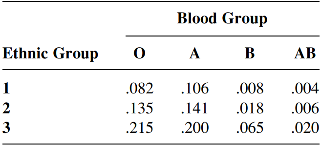
Suppose that an individual is randomly selected from the population and define the events \(A=\) type A selected, \(B=\)type B selected and \(C=\)ethnic group 3 selected.

Calculate the probability \(P(A)\).
Calculate the probability \(P(A|C)\)
If the selected individual does not have type \(B\) blood, what is the probability that he or she is from ethnic group 1.

2.8 Bayes’ Theorem

Consider an experiment of rolling a die and define the two events:

\(E=\) the event of observing an even number \(E^c\) the event of observing an odd number

Taken together, event \(E\) and \(E^c\) make up the sample space \(S\), consisting of all the possible number of points facing up, that is \(\{1,2,3,4,5,6\}\). Since a prime number can be either even (2) or odd(1,3,5), the event \(B\), which is that the number facing up is a prime number consists of both those simple events in \(B\) and \(E\) and those simple events in \(B\) and \(E^c\). Since these two events are mutually exclusive, we can write the event \(B\) as

\[ \begin{aligned} B=(B\cap E)\cup(B\cap E^c) \end{aligned} \] and

\(P(B)=P(B\cap E)+P(B\cap E^c)=1/6+3/6=2/3=0.6667\)

Suppose now that the sample space can be partitioned into \(k\) sub-populations, \(A_1,A_2,\dots,A_k\), that are mutually exclusive and exhaustive. Events are said to be exhaustive if one \(A_i\) must occur, such that \(A_1\cup A_2\cup\dots\cup A_k=S\). As above, the event \(B\) can be expressed as \[ \begin{aligned} B=(B\cap A_1)\cup(B\cap A_2)\cup\dots\cup(B\cap A_k) \end{aligned} \] Then,

\[ \begin{aligned} P(B)=P(B\cap A_1)+P(B\cap A_2)+\dots+P(B\cap A_k) \end{aligned} \] This is illustrated in Figure 2.7.

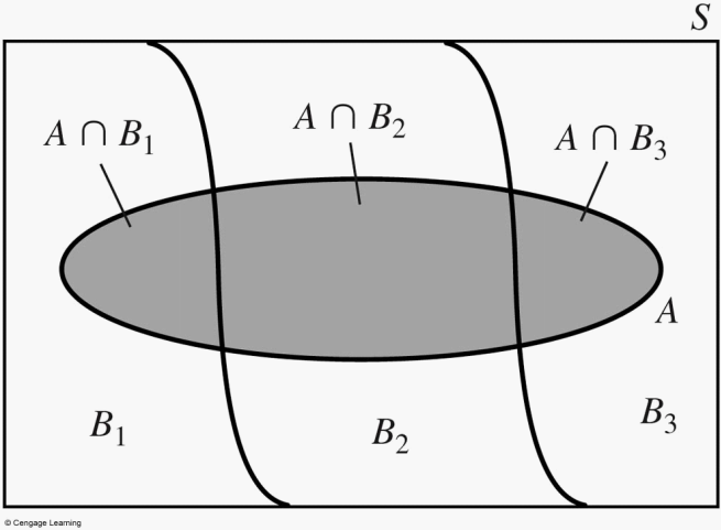
Figure 2.7: Decomposition of the event \(B\)

We can go one step further and use the multiplication rule to write \(P(B\cap A_i)=P(B|A_i)P(A_i)\), for \(i=1,2,\dots,k\). The result is known as the law of total probability.

Definition 2.1 (Law of Total Probability) Let \(A_1,A_2,\dots,A_k\) be mutually exclusive and exhaustive events. Then for any event \(B\), \[\begin{eqnarray} P(B)&=&P(B\cap A_1)+P(B\cap A_2)+\dots+P(B\cap A_k)\\ &=&\sum^k_{i=1}P(B|A_i)P(A_i) \end{eqnarray}\]

Example 2.20 (Oil Change) The members of a consulting firm rent cars from three rental agencies:

\(60\%\) from agency 1
\(30\%\) from agency 2
\(10\%\) from agency 3

\(9\%\) of the cars from agency 1 need an oil change, \(20\%\) of the cars from agency 2 need an oil change and \(6\%\) of the cars from agency 3 need an oil change. Calculate the probability that a rental car delivered to the firm will need an oil change.

Solution:

Let \(B=\) the event that a rental car needs an oil change

We have the partition:

\(A_1=\) the event that a car comes from agency 1
\(A_2=\) the event that a car comes from agency 2
\(A_3=\) the event that a car comes from agency 3

We have the following probabilities:

By the law of total probability, the probability that a rental car delivered to the firm will need an oil change is: \[\begin{eqnarray} P(B)&=&P(B|A_1)P(A_1)+P(B|A_2)P(A_2)+P(B|A_3)P(A_3)\\ &=&0.09(0.6)+0.2(0.3)+0.06(0.1)\\ &=&0.12 \end{eqnarray}\]

Now, suppose that we know that a car delivered to the firm needs an oil change, what is the probability that the rental car came from Agency 2? This probability can be obtained by the Bayes’ Theorem.

Definition 2.2 (Bayes' Theorem) Let \(A_1,A_2,\dots,A_k\) be mutually exclusive and exhaustive events with \(P(A_i)>0\), for \(i=1,2,\dots,k\). Then for any event \(B\), where \(P(B)>0\),

\(P(A_j|B)=\frac{P(A_j\cap B)}{P(B)}=\frac{P(B|A_j)P(A_j)}{\sum^k_{i=1}P(B|A_i)P(A_i)}\) for \(j=1,2,\dots,k\)

Now, we return to the above question.

Example 2.21 (Oil Change-Continued) Suppose that we know that a rental car delivered to the firm needs an oil change, what is the probability that the rental car came from Agency 2?

Solution:

\[ \begin{eqnarray} P(A_2|B)&=&\frac{P(B|A_2)P(A_2)}{P(B|A_1)P(A_1)+P(B|A_2)P(A_2)+P(B|A_3)P(A_3)}\\ &=&\frac{0.2(0.3)}{0.09(0.6)+0.2(0.3)+0.06(0.1)}\\ &=&\frac{0.06}{0.12}\\ &=&\frac{P(B\cap A_2)}{P(B)}\\ &=&0.50 \end{eqnarray} \] - Recall that \(P(A_2)\), the probability that a rental car comes from Agency 2 is \(0.3\) - Given that it needs an oil change, the new

Exercises

A sample is selected from one of two populations, \(S_1\) and \(S_2\), with \(P(S_1)=0.7\) and \(P(S_2)=0.3\). The probabilities that an event \(A\) occurs, given \(P(A|S_1)=0.2\) and \(P(A|S_2)=0.4\), calculate

\(P(A)\), using the Law of Total probability.
\(P(S_1|A)\) using Bayes’ theorem.

A population can be divided into two subgroups that occur with probabilities \(60\%\) and \(40\%\), respectively. An event \(A\) occurs \(30\%\) of the time in the first subgroup and \(50\%\) of the time in the second subgroup. What is the probability of the event \(A\), regardless of which subgroup it comes from?
Hatfield crime records show that \(20\%\) of all crimes are violent and \(80\%\) are non-violent, involving theft, forgery, and so on. Ninety percent of violent crimes are reported versus \(70\%\) of non-violent crimes.

What is the overall reporting rate for crimes in Hatfield?
If a crime in progress is reported to the police, what is the probability that it is violent? What is the probability that it is nonviolent?

Suppose that, in Gauteng, \(45\%\) of all matric finalists go to the University of Pretoria, \(35\%\) go to the University of Wits and \(20\%\) go to the University of Johannesburg. The pass rates for weapons at the three universities are \(0.9\), \(0.8\) and \(0.85\), respectively. If a student at one of the Universities passes, what is the probability that the student went to the University of Pretoria? University of Wits?